Count-Min Sketch
Let’s say we want to count the number of times elements appear in a stream of data. A simple solution is to maintain a hash table that maps elements to their frequencies.
This approach does not scale: Imagine having a stream with billions of elements, most of which are unique. Even if we are only interested in the most important ones, this method has huge space requirements. Since we do not know for which items to store counts, our hash table will grow to contain billions of elements.
The Count-Min Sketch, or CMS for short, is a data structure that solves this problem in an approximate way. Similarly to Bloom Filters, we save a lot of space by using probabilistic techniques. In fact, a CMS works a bit like a Counting Bloom Filter, though they do have different use cases.
Approximate Counts with Hashing
Given that we only have limited space availability, it would help if we could get away with not storing elements themselves but just their counts. To this end, let’s try to use only an array, with \( w \) memory cells, for storing counts.
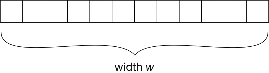 |
With the help of a hash function h, we can implement a counting mechanism based on this array. To increment the count for element \( a \), we hash it to get an index into the array. The cell at the respective index \( h(a) \) is then incremented by \( 1 \).
Concretely, this data structure has the following operations:
- Initialization: \( \forall i \in \{1, \dots, w\}: \operatorname{count}[i] = 0 \)
- Increment count (of element \( a \)): \(\operatorname{count}[h(a)] \mathrel{+}= 1 \)
- Retrieve count (of element \( a \)): \(\operatorname{count}[h(a)]\)
This approach has the obvious drawback of hash conflicts. We would need a lot of space to make collisions unlikely enough to get good results. However, we at least do not need to explicitly store keys anymore.
More Hash Functions
Instead of just using one hash function, we could use \( d \) different ones. These hash functions should be pairwise independent. To update a count, we then hash item \( a \) with all \( d \) hash functions, and subsequently increment all indices we got this way. In case two hash functions map to the same index, we only increment its cell once.
Unless we increase the available space, of course all this does for now is to just increase the number of hash conflicts. We will deal with that in the next section. For now let’s continue with this thought for a moment.
If we now want to retrieve a count, there are up to \( d \) different cells to look at. The natural solution is to take the minimum value of all of these. This is going to be the cell which had the fewest hash conflicts with other cells.
\[\min_{i=1}^d \operatorname{count}[h_i(a)]\]While we are not fully there yet, this is the fundamental idea of the Count-Min Sketch. Its name stems from the process of retrieving counts by taking the minimum value.
Fewer Hash Conflicts
We added more hash functions but it is not evident whether this helps in any way. If we use the same amount of space, we definitely increase hash conflicts. In fact, this implies an undesirable property of our solution: Adding more hash functions increases potential errors in the counts.
Instead of trying to reason about how these hash functions influence each other, we can design our data structure in a better way. To this end, we use a matrix of size \(w \times d\). Rather than working on an array of length \( w \), we add another dimension based on the number of hash functions.
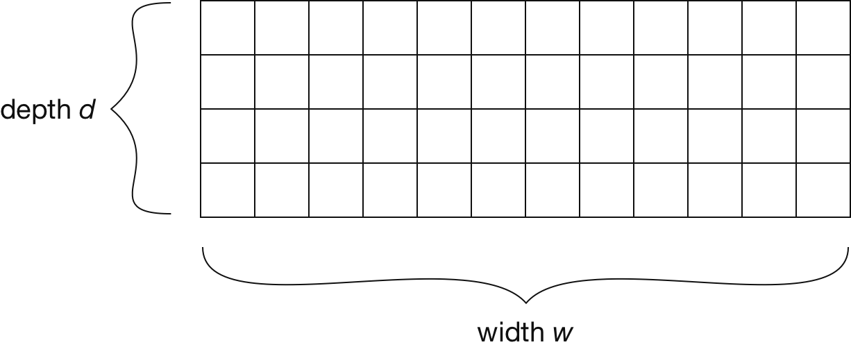 |
Next, we change our update logic so that each function operates on its on row. This way, hash functions cannot conflict with another anymore. To increment the count of element \( a \), we now hash it with a different function once for each row. The count is then incremented in exactly one cell per row.
- Initialization: \( \forall i \in \{1, \dots, d\}, j \in \{1, \dots, w\}, : \operatorname{count}[i, j] = 0 \)
- Increment count (of element \( a \)): \( \forall i \in \{1, \dots, d\}: \operatorname{count}[i, h_i(a)] \mathrel{+}= 1 \)
- Retrieve count (of element \( a \)): \(min_{i=1}^d \operatorname{count}[i, h_i(a)]\)
This is the full CMS data structure. We call the underlying matrix a sketch.
Guarantees
The counts we retrieve from a CMS data structure are approximate by nature. However, there are some theoretical guarantees on error bounds. The parameters \( w \) and \( d \) can be configured so that errors are of reasonable magnitude for the application at hand.
We can start off by stating that CMS can only overestimate counts, i.e. the frequencies it returns are upper bounds. Errors are only introduced when cell values are incremented too much because of hash conflicts. Thus, it is not possible that the returned count is too low.
To describe the bounds on how much CMS overestimates, we can use two variables, \( \epsilon \) and \( \delta \). Additionally, let \( ||\operatorname{count}||_1 \) be the sum of all counts stored in the data structure, i.e. the sum of values in one row of the sketch. The central guarantee CMS provides is then the following:
Theorem: With a probability of \( 1 - \delta \), the error is at most \( \epsilon * ||\operatorname{count}||_1 \). Concrete values for these error bounds \( \epsilon \) and \( \delta \) can be freely chosen by setting \( w = \lceil e / \epsilon \rceil \) and \( d = \lceil \ln(1 / \delta)\rceil \).
The full proof of this result is given in original CMS paper [1] . Adding another hash function quickly reduces the probability of bad errors which are outside the bound. This is because hash conflicts would now also need to appear in the new row, additionally to all the previous rows. Since the hash functions are pairwise independent, this has an exponential effect. Increasing the width helps spread up the counts, so it reduces the error a bit further, but only has a linear effect.
Typically the sketch is much wider than it is deep. Using many hash functions quickly becomes expensive. It is also not necessary to add a large number of hash functions since \( \delta \) rapidly shrinks as we add more rows.
Applications
Generally, CMS is useful whenever we only care about approximate counts of the most important elements. A property that allows for many applications is that it is possible to first fill the data structure, and then later query it with valid keys. In other words, we initially do not need to know the keys we are actually interested in.
Database Query Planning
Database engines plan how they execute queries. How quickly a query is performed can heavily depend on the execution strategy, so it is a crucial area of optimization. For example, this is especially important when determining the order in which several joins are performed, a task known as join order optimization.
Part of finding good execution strategies is estimating the table sizes yielded by certain subqueries. For example, given a join, such as the one below, we want to find out how many rows the result will have.
SELECT *
FROM a, b
WHERE a.x = b.x
This information can then be used to allocate a sufficient amount of space.
More importantly, in a bigger query where the result is joined with a table c, it could be used to determine which tables to join first.
To estimate the size of the join, we can create two CM sketches.
One holds the frequencies of elements x in a, the other holds frequencies of elements x in b.
We can then query these sketches to estimate how many rows the result will have.
Building up full hash tables for this task would require a huge amount of space. Using a sketch data structure is much more feasible, especially since the SQL tables in the join could potentially be very big. Furthermore, an approximate result is generally good enough for planning.
Finding Heavy Hitters
A common task in many analytics application is finding heavy hitters, elements that appear a lot of times. For example, given a huge log of website visits, we might want to determine the most popular pages and how often they were visited. Again, building up a full hash table could scale badly if there is a long tail of unpopular pages that have few visits.
To solve the problem with CMS, we simply iterate through the log once and build up the sketch [2] . To query the sketch, we need to come up with candidate keys to check for. If we do not have an existing candidate set, we can simple go through the log again and look up each page in the CMS, remembering the most important ones.
Beyond Point Queries
The type of queries discussed in this blog points are point queries, i.e. estimates of the counts of individual items. However, CMS also allows for more advanced queries. These include range queries and inner product queries, which could be used to compute even better estimates of join sizes.
Summary
To summarize, the Count-Min Sketch is a probabilistic data structure for computing approximate counts. It is useful whenever space requirements could be problematic and exact results are not needed. The data structure is designed in a way that allows freely trading off accuracy and space requirements.