Reservoir Sampling
One of my favorite algorithms is part of a group of techniques with the name reservoir sampling. I like how the algorithm is neither complex nor requires fancy math but still very elegantly solves its problem. Incidentally, it also happens to be the solution to a popular interview question.
The problem goes like this: Given a stream of elements, we want to sample \(k\) random ones, without replacement and by using uniform probabilities. The total number of elements in the stream is unknown. At any point, someone could stop the stream, and we have to return k random elements. This blog post goes over a naive solution first, followed by one that actually scales, and then finally the algorithm that I find so elegant.
Naive Approach
If we do not know how to solve the problem, we could try to reduce it to one that we do know how to solve. To this end, we could store all elements of the stream in an array. The problem then reduces down to sampling \(k\) random indices, whose respective elements are returned.
Clearly, this method does not scale. The stream might contain billions of elements and we do not want to, and often cannot, keep all of them in memory. Furthermore, we essentially solve the problem in two distinct steps. First we build up an array of all elements, then we try to select random ones. This does not seem like a natural solution to such a streaming problem.
Random Tags
Sorting
Still, let’s keep going with this idea for a moment. If we are already storing all elements of the stream, we could just as well sort them randomly. To do this, we assign a random tag to each element, a random number between 0 and 1. We then sort by the random tag and keep the \(k\) smallest items.
Of course, this does not scale any better. It also does not improve on the space requirement at all. We essentially still duplicate the stream to be able to sort it.
Reservoir
However, there is an obvious bottleneck to the solution above. We are sorting the entire stream, even though we in fact only care about \(k\) elements. In a lot of cases, \(k\) will be much smaller than the total number of elements in the stream, so we are performing a lot of unnecessary work.
To improve on this, let’s think about the case of \(k = 1\). If we only care about one random element, then we should only keep track of the element with the smallest tag. The other elements can be discarded as we iterate over the stream.
For arbitrary \(k\), we should keep track of a reservoir of the \(k\) elements with the smallest tags. Naively, we can do this by comparing the random tag of the current element to the random tags of elements in the reservoir. If necessary, the element with the largest tag is then replaced.
Heaps
This works, but at this stage the problem calls for using a heap for better complexity. Heaps exactly solve the problem of keeping track of the \(k\) smallest elements in an efficient way. This solution is much better: We do not need any additional space, and when we process a new element, we at most have \(\mathcal{O}(\log k)\) work to perform.
An additional advantage of the new solution is that we have a valid sample available after each step of the stream. This makes it possible to use the sampling technique in applications where the stream might continue indefinitely. For example, think of a web server that receives requests and should at any point be able to provide a sample of those requests. As users send more data to the server, the sample changes. Still, at any point the server is able to provide such a sample, without keeping track of every request ever sent.
Adapting Probabilities
The solution we arrived at is nice, but we can do even better. It is possible to bring the logarithmic factor down to a constant one. We now discard the idea of random tags but still make use of a reservoir of \(k\) elements.
Instead of structuring the reservoir in a certain way, e.g. by using a heap, we are going to use an array. As we process the stream, we replace items in the reservoir with a certain probability. This probability is adapted as we keep on iterating over the stream [1] .
Let’s again start with the base case of \(k = 1\). The final algorithm for sampling this element works as follows:
- Store the first element as the reservoir element
- For the \(i\)-th element, make it the reservoir element with a probability of \(1 / i \)
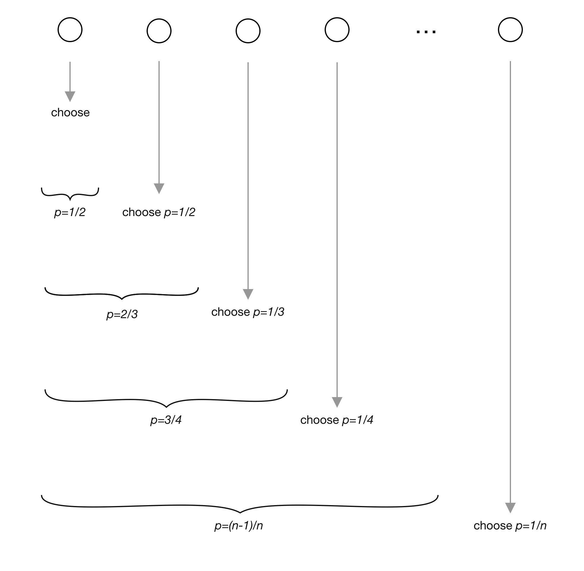
This is the algorithm that I find so elegant. It is incredibly simple, has perfect complexity, and yet the way it works seems to be a bit magical. If we think about some examples, adapting the probabilities like this seems to just work out. For example, we would process a stream with three elements as follows:
- Store the first element
- Store the second element with a probability of \(1 / 2\). Now both elements have equal probabilities of being in the reservoir
- Store the third element with a probability of \(1 / 3\). The previous two elements also have a final probability of \((1 / 2) * (2 / 3) = 1 / 3\) to be chosen
The following visualization shows this. Circles represent the elements in the stream.
 |
Proof
It turns out that by induction this works for any number of elements.
Base case: The algorithm trivially works for \(n = 1\).
Induction assumption: For a stream with \(n\) elements, all elements are chosen with the same final probability \(1/n\).
Inductive step: \(n \rightarrow n + 1\). We want to show that for a stream of \(n + 1\) elements, all items still have the same probability of \(1 / (n + 1)\) to be sampled.
The algorithm tells us to choose the next element of the stream with a probability of \(1 / (n + 1)\). All other elements can be the current reservoir element with a probability of \(1 / n\) by the induction assumption.
The current reservoir element has a probability of \(1 - 1 / (n + 1) = n / (n + 1)\) to stay. This means all previous elements have a final probability of \((1 / n) * (n / (n + 1)) = 1 / (n + 1)\) to be the reservoir element after this step. Thus, all elements still have the same probability of being selected as the reservoir element.
Sampling \(k\) Elements
If we want to sample \(k\) random elements using this technique, we need to adapt the algorithm slightly. We again keep a reservoir of \(k\) elements. This reservoir is initialized to contain the first \(k\) elements of the stream.
When processing the \(i\)-th element for \(i > k\), we add it to the reservoir with a probability of \(k / i\). If we add it, we do that by replacing a random element of the reservoir. In other words, in that case each element of the reservoir has a probability of \(1 / k\) to be replaced. The value of \(k / i\) is derived from the fact that this is the probability that any given element is sampled from a uniform distribution if we want to select \(k\) items.
Full algorithm:
- Store the first \(k\) elements as the reservoir elements
- For the \(i\)-th element, add it to the reservoir with a probability of \(k / i\). This is done by replacing a randomly selected element in the reservoir
The proof of the algorithm again works out by induction. Since the arithmetics get a bit more finicky for the case of \(k \neq 1\), I have put the full proof into the appendix.
Applications
Sampling From Streams
Generally speaking, reservoir sampling is useful whenever we sample from a stream and do not know how many elements to expect. In programming, this translates into sampling from any iterable.
Operations in Spark are a nice example to illustrate this on: Let’s say we apply a filter to a stream of data and then sample from the result. A naive solution is to first run the filter, then count the number of elements, and finally use that result to sample.
However, if we use reservoir sampling, the query optimizer can compress all of this into one step. As an item is processed, the filter function is first applied, and if necessary it is afterwards decided if the element should be kept in a reservoir.
If the elements are read from disk and then directly sampled, one could even optimize the deserialization process. Only elements that reservoir sampling selects would need to be deserialized. Reservoir sampling is a natural fit for both these applications since we do not know how many elements the streams will contain.
Database Query Planning
Database engines plan how to execute queries. To do this, the query is optimized and several different execution strategies are considered. To decide on one, we can run simulations by executing them on subsets of the data [2] .
Reservoir sampling can be used to sample such a subset. Depending on how the data is read, we might not know beforehand how much data there is in total. Furthermore, reservoir sampling makes it possible to easily add the sampling process to only specific parts of the query.
Summary
Reservoir sampling allows us to sample elements from a stream, without knowing how many elements to expect. The final solution is extremely simple, yet elegant. It does not require fancy data structures or complex math but just an intuitive way of adapting probabilities. Proofing that it works also seems like a good example for learning about induction.
The solution of adapting probabilities is optimal for the problem as described here. However, there are various extensions for different use cases. The random tag algorithm can be extended to make it possible to sample from weighted distributions. Additionally, if the iterable interface allows skipping a certain number of items, the algorithm of adapting probabilities can be improved further. The final complexity then depends on how many elements we want to sample, rather than just on how many elements the stream has.
References
- Vitter, J. S. (1985). Random sampling with a reservoir. ACM Transactions on Mathematical Software (TOMS), 11(1), 37-57.
- Cormode, G. (2017). What is Data Sketching, and Why Should I Care?. Communications of the ACM (CACM), 60(9), 48-55.
Appendix
Proof for sampling \(k\) elements
Base case: The algorithm trivially works for \(n = k\).
Induction assumption: For a stream with \(n\) elements, and for \(k \le n\), all elements are chosen with the same final probability \(k/n\).
Inductive step: \(n \rightarrow n + 1\)
Equivalently to before, the algorithm tells us to choose the next element of the stream with a probability of \(k / (n + 1)\). All other elements can be the current reservoir element with a probability of \(k / n\) by the induction assumption.
To compute the probability of an element being kept in the reservoir, we need to consider two cases:
- The current element of the stream is not added to the reservoir at all: \(1 - (k / (n + 1)) = (n + 1 - k) / (n + 1)\)
- (a) It is added but (b) does not replace the element in the reservoir we are considering
- (a): \(k / (n + 1)\)
- (b): \(1 - (1 / k) = (k - 1) / k\)
- Joint probability: \((k / (n + 1)) * ((k - 1) / k) = (k - 1) / (n + 1)\) This is the result of multiplying (a) and (b)
We need to add these two cases since they are fully disjoint: \[ (n + 1 - k) / (n + 1) + (k - 1) / (n + 1) = n / (n + 1) \]
This is the probability of an element staying in the reservoir. Finally, each previous element had a chance of \(k / n\) to be in the reservoir to begin with. The prior steps were independent of the current one, so we have to multiply the two probabilities: \[ (n / (n + 1)) * (k / n) = k / (n + 1) \]
And this is exactly where we wanted to arrive at. All elements still have the same final probability of ending up in the reservoir.