RProp
RProp is a popular gradient descent algorithm that only uses the signs of gradients to compute updates [1] [2] . It stands for Resilient Propagation and works well in many situations because it adapts the step size dynamically for each weight independently. This blog posts gives an introduction to RProp and motivates its design choice of ignoring gradient magnitudes.
Most gradient descent variants use the sign and the magnitude of the gradient. The gradient points in the direction of steepest ascent. Because we typically want to find a minimum, we follow the gradient in the opposite direction. This direction is completely determined by the sign of the gradient.
Gradient magnitudes
To decide on the step size, a scaled version of the gradient’s magnitude is generally used by most gradient descent algorithms. This heuristic often works well but there is no guarantee that it is always a good choice. To see that it can work extremely badly, and does not have to contain valuable information, we consider a function \(f\). The plots below show \(f\) as well as two scaled versions.
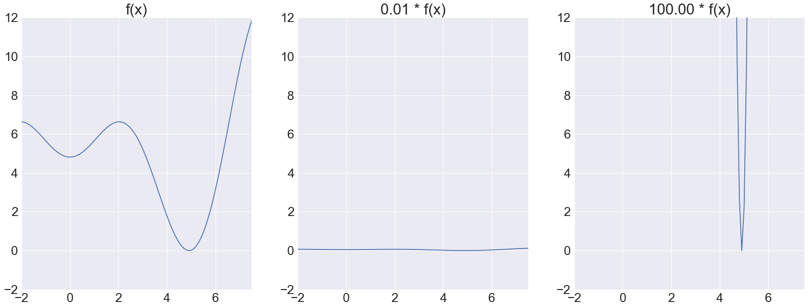 |
All three of these functions have the exact same optima, so the step updates using gradient descent should all be similar. However, if we determine the step size using the gradient’s magnitude, then the step sizes for the three functions differ by orders of magnitude. Even worse, the gradient virtually vanishes for the second function and explodes for the third, as shown below:
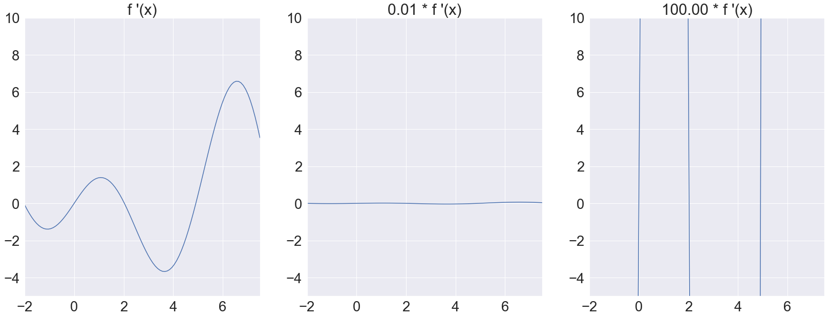 |
This shows that the gradient’s magnitude does not necessarily contain useful information for determining the step size. Even though optima can still be found by choosing appropriate learning rates, this makes it clear that using the gradient’s magnitude at all is sometimes questionable. Using a fixed learning rate will also fail if only some parts of the function are scaled.
Updating weights
Modern gradient descent variants try to circumvent this problem by dynamically adapting the step size. RProp does this in a way that only requires the sign of the gradient. By ignoring the gradient’s magnitude, RProp has no problems if a function has a few very steep areas.
Concretely, RProp uses a different step size for each dimension. Let \(\eta_i^{(t)}\) be the step size for the \(i\)-th weight in the \(t\)-th iteration of gradient descent. The value for the first and second iteration, \(\eta_i^{(0)}\) and \(\eta_i^{(1)}\), is a hyperparameter that needs to be chosen in advance. This step size is then dynamically adapted for each weight, depending on the gradient.
The weights themselves are updated using
\[w_i^{(t)} = w_i^{(t - 1)} - \eta_i^{(t - 1)} * \operatorname{sgn}\left(\frac{\partial E^{(t - 1)}}{\partial w_i^{(t - 1)}}\right)\]where the sign of the partial derivative of the error in the last step with respect to the respective weight is computed. We go in the direction of descent using the determined step size.
Adapting the step size
In each iteration of RProp, the gradients are computed and the step sizes are updated for each dimension individually. This is done by comparing the gradient’s sign of the current and previous iteration. The idea here is the following:
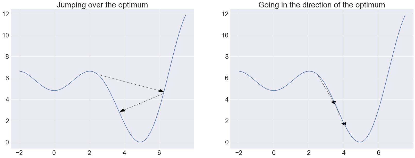
- When the signs are the same, we go in the same direction as in the previous iteration. Since this seems to be a good direction, the step size should be increased to go to the optimum more quickly
- If the sign changed, the new update is moving in a different direction. This means that we just jumped over an optimum. The step size should be decreased to avoid jumping over the optimum again
A visualization of this idea is shown below.
 |
To implement this update scheme, the following formula is used:
\[\eta_i^{(t)} = \begin{cases} \min(\eta_i^{(t - 1)} * \alpha, \eta_{\max}) & \text{if } \frac{\partial E^{(t)}}{\partial w_i^{(t)}} * \frac{\partial E^{(t - 1)}}{\partial w_i^{(t - 1)}} > 0 \\ \max(\eta_i^{(t - 1)} * \beta, \eta_{\min}) & \text{if } \frac{\partial E^{(t)}}{\partial w_i^{(t)}} * \frac{\partial E^{(t - 1)}}{\partial w_i^{(t - 1)}} < 0 \\ \eta_i^{(t - 1)} & \text{otherwise} \end{cases} \label{eq:rprop}\]where \(\alpha > 1 > \beta\) scale the step size, depending on whether the speed should be increased or decreased. The step size is then clipped using \(\eta_{\min}\) and \(\eta_{\max}\) to avoid it becoming too large or too small. If a gradient was zero, a local optimum for this weight was found and the step size is not changed.
Hyperparameters
These seem like many hyperparameters to choose, but in practice there are known values for them that generally work well. It is also not problematic if the clipping values \(\eta_{\min}\) and \(\eta_{\max}\) are respectively smaller and larger than necessary because an inconvenient step size is generally adapted quickly.
Popular values for \(\alpha\) and \(\beta\) are \(1.2\) and \(0.5\). Heuristically, it works well to increase the step size slowly, while allowing for the possibility of quickly decreasing it when jumping around an optimum. For fine-tuning the weights, it is important that \(\beta\) is not the reciprocal of \(\alpha\), to allow for many different step sizes.
Conclusion
One advantage of RProp that was not discussed so far is having a different step size for each weight. If one weight is already very close to its optimal value while a second weight still needs to be changed a lot, this is not a problem for RProp. Other gradient descent variants can have much more problems with such a situation, especially because the gradient magnitudes can be misleading here.
While RProp works well in a lot of situations, it is not perfect. For instance, RProp generally requires large batch updates. If there’s too much randomness in stochastic gradient descent, then the step sizes jump around too much and the updates work badly.
Implementing RProp is quite straightforward. To get a better understanding of RProp, reading the PyTorch implementation can also be helpful.